W01 Learning Activity: Evaluating Performance
Overview
To evaluate code and look for alternative solutions, it is important that we have a common method for quantifying the performance of code in terms of time. The principles we will learn can also be applied to analysis of how much memory or space is used by code to perform a task.
Big O Notation and Linear Performance
Big O notation is used to describe the performance of an algorithm (or function) for large sets of data. If we have two functions that do the same thing, we can use big O notation to compare the performance of the two functions. As a simple example, consider the following code which looks for the name "Bob" in a list of names:
bool FindBob(List nameList)
{
  foreach (var name in nameList)
  {
    if (name == "Bob")
    {
      return true;
    }
  }

  return false;
}
The size of the data in this function is based on the size of the nameList. We will say that size of
the data is n. The for loop in the code means that we will potentially run n times. This
worst case potential will only happen if "Bob" is not in the list of names. Therefore, we say that the big O in
the worst case is O(n). In general, when we ask for the big O of a function we are asking for the worst case
scenario. This function does have a best case scenario. If "Bob" is the first name in the list, then the loop will
only run one time. Therefore, we can say the big O in the best case is O(1). We call O(1)
constant time. When looking at code, usually a single line of code like an assignment statement
is considered O(1).
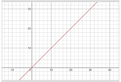
If a function has O(n) performance, then we also say that the function has linear performance. Using a graphing calculator or a graphing website, we can visually see the linear performance of O(n). The graph below shows y = x which is used to represent O(n). When x (or n) gets bigger, the amount of work (y) gets larger in a linear way.
Consider the following code that has two loops in serial (one right after the other):
void MultipleLoops(int n)
{
  for (int i = 0; i < n; i++)
  {
    Console.WriteLine(i);
  }

  for (int j = 0; j < n; j++)
  {
    Console.WriteLine(j*j);
  }
}
In this function, each for loop contributes O(n) to the performance of the function. The total would
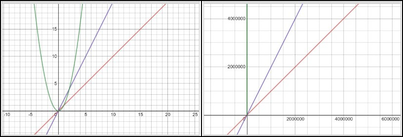
be O(n) + O(n) = O(2n). If we graph this, O(2n) does look like it has a worse performance than O(n). However, if
we zoom very far out to very large values of n, it is still just two times more work. If we graphed
O(n2) for these large values, we can't even see the line escape the y-axis. O(n) and O(2n) are
equivalent. Any coefficients in big O notation should be dropped. Therefore, instead of saying
O(2n) for the function above, we will say O(n).
Polynomial Performance
As seen earlier, the structure of the for loops is important to analyzing the big O performance for a function. Consider the following scenario:
void MultiplicationTable(int n)
{
  for (int i = 0; i < n; i++)
  {
    for (int j = 0; j < n; j++)
    {
        Console.WriteLine((i + 1) * (j + 1));
    }
  }
}
This function has a loop within a loop. Both loops are based on the size of the data. Instead of adding O(n)
twice like we did with loops in serial, we multiply as follows: O(n) * O(n) = O(n2). The rate of
increase is much higher with an O(n2) function compared to an O(n) function. The FindBob
function would, in the worst case, take 1,000 checks if the list size was 1,000, but the
MultiplicationTable will take 1,0002 = 1,000,000 print statements to complete for a
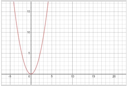
similarly sized value of n. This results in O(n2) which is polynomial time. The graph
for an O(n2) function is shown below:
Caution should be used when analyzing code that contains a loop within a loop. If one of the loops is based on
the size of the data but the other loop is not, it would be more accurate to characterize it as O(kn) where
k is a constant. Based on the rules we learned earlier, O(kn) = O(n) when k is a
coefficient. The code below would be O(n) because the inner loop is only running three times but the outer loop is
based on the size of the data.
void ShortMultiplicationTable(int n)
{
  for (int i = 0; i < n; i++)
  {
    for (int j = 0; j < 3; j++)
    {
        Console.WriteLine((i+1) * (j+i));
    }
  }
}
When we count iterations of a loops in a function, we may end up with complex polynomials that look like this. Assume that we had performance predicted at O(2n3 - 7n2 + 13n - 15). In addition to dropping coefficients, we also drop lesser exponents like (in this example) the n2 and the n. Therefore, O(2n3 - 7n2 + 13n - 15) = O(n3). This code likely has a loop, within a loop, within a loop.
Logarithmic Performance
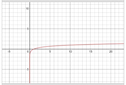
It would seem like O(n) is the best performance you can get if we want to analyze a set of information. However, there are some algorithms that have better performance. Consider a function that had performance of O(log n). This is called logarithmic time. When graphed, the performance does not get significantly worse as the size of the data increases.
To find a function that has this type of performance, consider a list of sorted data: 2, 7, 12, 19, 31, 54, 68, and 91. If we wanted to determine if 68 was in the list, we could search from left to right looking for 68. Instead, we are going to treat this sorted list of numbers like a phone book. If we wanted to find a name in a phone book, we would likely use our knowledge of the alphabet to get there faster. A simple process could be to go to the item in the middle of the list (or the phone book) and determine if the number we are looking for is before or after the value in the middle. By doing this, we will discard half of the values in the list in support of our search. Using the remaining numbers, we will repeat the process by going to the middle and discarding half again. If we repeat this process, we will eventually either find the number or determine that the number does not exist.
Returning to our list of numbers, we will say 19 is in the middle (we started with an even number so we will use
integer division to find the middle such as numbers.Count / 2. Since 68 (the number we are looking
for) is greater than 19, then we concentrate our search after the 19. The middle of the remaining numbers (31, 54,
68, and 91) is 54. Since 68 is greater than 53, we will look at the numbers afterwards. The middle of the
remaining numbers (68 and 91) is 68. Since 68 matches 68, we can say the number exists and it only took us three
checks.
If we look at this generically, let's ask ourselves how many checks it will take if we had n numbers
in the list. The worst case would occur if the number we are looking for is not in the list. Therefore, we want to
know how many checks it will take (in terms of n) until we reach the point where there is only one
item left in the list to check (because that means we don't have to look any further). To solve this problem,
consider how many numbers are left after each check.
- After check 1, we have
n/ 2 left - After check 2, we have
n/ 4 left - After check 3, we have
n/ 8 left - Generally, after check c, we have
n/ (2c) left
Returning to the question, how many checks c are there until there is just one left. Written
mathematically: n/(2c) = 1. Using logarithms, we get c = log2(n) =
log(n) / log(2) which results in a big O notation of O(log n) since the log(2) is a coefficient. The secret to
getting O(log n) was to continuously divide the data in half.
The process above relies on an important fact. The ability to find the middle of a list (or dynamic array as you learned previously) using a lookup operation is O(1). The next section will review why this is true.
Performance of Dynamic Arrays
Now that we have big O notation, we can characterize the performance of our data structure operations.
| Function | Description | Performance |
|---|---|---|
| lookup(index) | Performance of getting a value in the dynamic array using the index. Since the dynamic array is in
contiguous memory, the equation address = startingAddress + (itemSize * index) can be used to
get the value in a dynamic array using the index quickly. |
O(1) |
| append(value) | Performance of adding to the end of dynamic array. If the dynamic array is not full yet, then the cost is based on the lookup operation to go to the next open space. If the dynamic array is full, then we need to create new memory which is twice the size and then copy the old memory. This is an O(n) operation because of the loop required. However, for large values of n, this copy doesn't happen very often. We can amortize (or spread out) the cost of the O(n) loop on all the previous appends that were filling up the dynamic array. Therefore, we say the worst case for appending in the dynamic array is O(1). | O(1) |
| insert(index, value) | Performance of inserting at the beginning or the middle of the dynamic array. When we insert anywhere but the end, then we will need a loop to move all the items from the index to the end over by one position. This requires a loop which in the worst case will require moving all items in the list. | O(n) |
| remove(index) | Performance of removing an element in the list. When we remove, we have to move all items over by one position towards the beginning of the list. This requires a loop that in the worst case will require moving all items in the list. However, in the case of removing the last item in the list, there is nothing to move over. This scenario will be O(1). | O(n); except for removing the last one which is O(1) |
| size() | Performance of returning the size of the dynamic array. The class for the dynamic array data structure will keep track of how many items are currently in the list so no loop is required. | O(1) |
| capacity() | Performance of returning the capacity of the dynamic array. The class for the dynamic array data structure will keep track of the capacity of the current list so no loop is required. | O(1) |
| empty() | Performance of checking the size of the dynamic array | O(1) |
Evaluating Performance of Alternative Solutions
The real benefit of using big O notation is to find a way to compare and contrast one or more functions that perform the same task. It is possible that we have written one function that functionally works very well. However, when we run the function, it is taking too long to complete. When code takes too long, the user may have a user interface that is unresponsive or the software may miss requests arriving from external sources. When this happens, we need to analyze the big O notation of our code and look for ways to improve it with a new function.
We should not be satisfied with the functionality of our code only. We should always consider the performance. In addition to looking at timing, we can also perform a similar analysis on the amount of memory our functions use. It is possible to write code in many different ways but not all solutions may have the best performance. We should always check the performance of our code especially when loops are involved. Care should be taken when multiple functions are used in software. If one function has a loop and calls another set of functions within that loop, the performance of the other functions needs to be considered to determine the big O of the calling function.
Measure Actual Execution Time
When we analyze performance, we are making a prediction. Frequently, we need to perform tests to
benchmark (or measure) the actual performance of the functions we are using. In C#, we
can use the System.Diagnostics.Stopwatch class to measure the execution time. Consider the following
example:
public void Run()
{
  var executionTime = Time(() => LotsOfLoops(100), 10);
  Console.WriteLine($"Execution Time: {executionTime} ms");
}

private void LotsOfLoops(int n)
{
  int total = 0;
  for (int i = 0; i < n; i++)
  {
    for (int j = 0; j < n; j++)
    {
      for (int k = 0; k < n; k++)
      {
          total += (i*j*k);
      }
    }
  }

  Console.WriteLine(total);
}

private double Time(Action executeAlgorithm, int times)
{
  var sw = Stopwatch.StartNew();
  for (var i = 0; i < times; ++i)
  {
    executeAlgorithm(); // Calls the action passed in to this method
  }

  sw.Stop();
  return sw.Elapsed.TotalMilliseconds / times;
}
We encapsulate all of the Stopwatch calls into the Time() function. The following may
help you understand this code better:
() => LotsOfLoops(100)in theRunfunction creates a function that will always callLotsOfLoopswith the parameter of100each time it's called. This is called a C#Actionand is received into theexecuteAlgorithmparameter in theTimefunction.Time(() => LotsOfLoops(100), 10);tells theTimefunction to execute theAction10 times.var sw = Stopwatch.StartNew();creates a newStopwatchobject and starts timing right away.sw.Stop();ends the timer and allows the program to get theElapsedtime.
Another way to look at actual performance is to instrument the code by adding a variable that counts how much work is performed. This variable can then be returned and compared to a base case for relative performance.
public void Run()
{
  var stopwatch = Stopwatch.StartNew();
  var work = LotsOfLoops(1000);

  stopwatch.Stop();

  // This will display 1000000
  Console.WriteLine("Innermost count is: {0}", work);

  // The time displayed will vary based on your computer
  Console.WriteLine("Execution Time in milliseconds: {0}", stopwatch.Elapsed.TotalMilliseconds);
}

private int LotsOfLoops(int n)
{
  int total = 0;
  int count = 0; // Variable for instrumentation

  for (int i = 0; i < n; i++)
  {
    for (int j = 0; j < n; j++)
    {
      for (int k = 0; k < n; k++)
      {
        total += (i*j*k);
        count++;  // Count the number of times in the inner-most loop
      }
    }
  }

  Console.WriteLine(total);

  return count;
}
Problem Solving Strategies
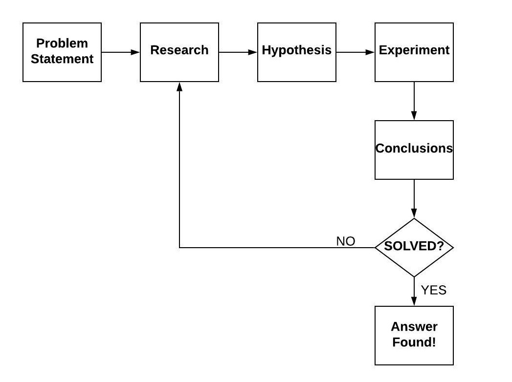
Scientific Method
It can be daunting to try to solve a problem (especially if you are constrained by time in an interview). While it can be tempting to either dive into code or dive into the internet to find help, we want to develop engineering discipline in our work. When we learned about science, we were introduced to the scientific method.
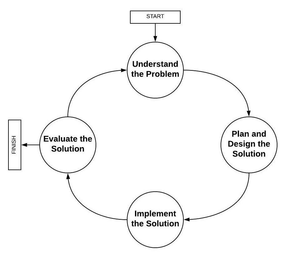
Four Step Process
When we go directly to writing code we are short-circuiting the process. When we start out the process by researching online but use the answers without experimenting with those ideas, we are also short-circuiting the process. For the purposes of solving problems with software, consider the following four steps that align well with the scientific method:
- Understand the Problem - Restate the problem in your own words. Ask questions to clarify the problem.
- Plan and Design the Solution - Brainstorm ideas and write them down. Try to solve the problem manually on paper. Consider if a data structure (for example, the dynamic array) could be used to solve the problem. Write down a design (for example, flow charts, block diagrams, pseudo-code, step-by-step process, etc).
- Implement the Solution - Using your design, implement the solution in a programming language.
- Evaluate the Solution - Test your solution on several example inputs. Identify which scenarios are working and which ones are not. If it is working, ask yourself if it could be done better (for example, faster, with less code, with fewer variables, etc). If the solution still needs work, return back to the first step again.
Video Discussion (Optional)
The following video is optional. It presents a brief discussion of the topic.
Activity Instructions
Determine the Big-O performance of each of the following. Once you have determined your answer, compare it to the provided solution:
-
static void DoSomething(int n)
{
  for (int i = 0; i < n; i++)
  {
    Console.WriteLine(n * n);
  }

  for (i = n; i > 0; i--)
  {
    Console.WriteLine(n * n * n);
  }
}
Solution (click to expand)
This function isO(n). Even though there are two loops, because they are not nested inside one another, the performance would beO(2n)which simplifies down toO(n)when the constant is dropped. -
static void DoSomethingElse(List<string> words)
{
  for (int i = 0; i < words.Count; i++)
  {
    for (int j = 0; j < words.Count; j++)
    {
      Console.WriteLine(".");
    }
  }
}
Solution (click to expand)
This function isO(n^2). Notice that in this case, the loops are nested and both depend on the variable "n" which is shorthand for the length of the list. -
static void DoAnotherThing(List<string> words)
{
  string sentence = "The quick brown fox jumps over the lazy dog";
  for (int i = 0; i < words.Count; i++)
  {
    for (int j = 0; j < sentence.Length; j++)
    {
      Console.WriteLine(".");
    }
  }
}
Solution (click to expand)
This function isO(n). This one is tricky, because there are two loops nested inside each other, but notice that only one of the loops depends on the variable n. The other depends on the length of the sentence which is a fixed constant. Thus, as the amount of words in the list gets large, it will dominate the constant factor added by iterating through the length of the sentence.
Key Terms
- algorithm
- A solution to a problem including the steps to solve the problem. An algorithm is implemented as one or more functions in code.
- benchmark
- The measurement of actual execution time of an algorithm as observed in multiple executions of the algorithm. Benchmarks are often taken within different environments (e.g. operating system, processor, programming language).
- big O
- A mathematical representation of the performance of an algorithm. As used in this lesson, it represents the
worst case execution time predicted for the code. Represented as a function in terms of
n, wherenrepresents the size of the data being processed by the code. - coefficient
- A numeric factor applied to a function. For example, O(2n) has a coefficient of 2 and O(5n2) has a coefficient of 5. In big O notation, the coefficient is dropped.
- constant
- An algorithm has constant time if it is not dependent on the size of data. Constant time is always reduced to O(1). A single expression in code is frequently O(1).
- linear
- An algorithm has linear time if the execution time increases at the same rate as the data size. Linear time is always reduced to O(n). Code that contains a single loop based on the size of the data is considered linear.
- logarithmic
- An algorithm has logarithmic time if the rate of growth decreases as the size of the data increases. Logarithmic time is commonly reduced to O(log n). Other variations include O(n log n). Logarithmic time is also described as the inverse of exponential growth (e.g. O(2n)). The practice of splitting data in half multiple times to achieve a goal is frequently considered logarithmic.
- performance
- Describes the amount of time and memory used to perform an algorithm in software. An algorithm can be implemented in many ways. However, the performance may be different between each implementation.
- polynomial
- An algorithm has polynomial time if the execution time increases by a fixed exponent relative to the size of the data. If a loop within a loop (both related to the size of data) were written, then the big O notation would be likely reduced to O(n2). If there were three embedded loops, the big O notation would be O(n3). Lower order exponents are dropped in big O notation. For example, O(4n3 + 7n2) = O(n3).
Submission
When you have finished all of the learning activities for the week, return to Canvas and submit the associated quiz there.
Other Links:
- Return to: Week Overview | Course Home