W09 Prepare: Reading
Table of Contents
Trees
Trees are like linked lists in that nodes are connected together by pointers. However, unlike linked lists, a tree can connect to multiple different nodes. We will look at the following types of trees: binary trees, binary search trees, and balanced binary search trees.
Binary Trees
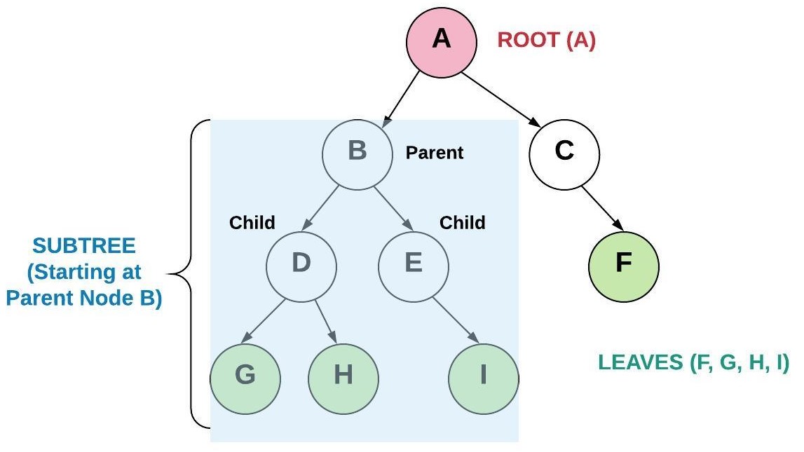
A binary tree is a tree that links to no more than two other nodes. In the picture below, the top node is called the root node. The nodes that connect to no other nodes are called leaf nodes. A node that has connected nodes is called a parent node. The node connected to the parent are called child nodes. The nodes to the left and right of any parent node form a subtree. There is always only one root node. While not shown in the picture, it is common for child nodes to also point back up to the parent node (similar to a linked list).
Binary Search Trees
A binary search tree (BST) is a binary tree that follows rules for data that is put into the tree. Data is placed into the BST by comparing the data with the value in the parent node. If the data being added is less than the parent node, then it is put in the left subtree. If the data being added is greater than the parent node, then it is put in the right subtree. If duplicates are allowed than the duplicate can be put either to the left or to the right of the root. By using this process, the data is stored in the tree sorted.
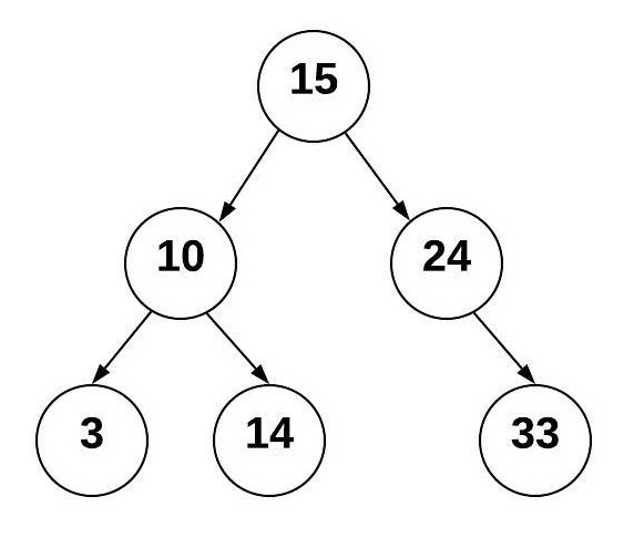
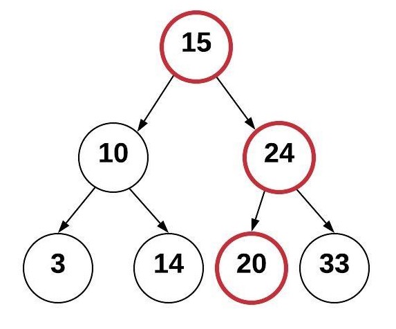
Using the tree above, we can determine where to put additional items. We always start at the root node and compare the new value with it. We keep comparing until we have found an empty place for the new node. For example, to insert the value 20, do the following:
Start at the root node 15 and compare with the new value 20
Since 20 is greater than 15, goto the right and visit node 24
Since 20 is less than 24, goto the left and see there is no additional node
Insert 20 in the empty spot to the left of 24.
The process that we used to find where to put the new node was an efficient process. If we had a dynamic array or a linked list containing sorted values, we would have an O(n) operation as we search for the proper location to insert a value into the proper sorted position. By using the BST, we are able to exclude a subtree with each comparison. This ability to split the job in half recursively results in O(log n). Maintaining sorted data in a BST performs better than other data structures.
However, the only reason we had O(log n) in the example above was because the tree was "balanced". To see the difference between a balanced and an unbalanced tree, we will construct a tree with the same values but in a different order. The reason why the previous tree has 15 as the root node is because 15 was added first. This time, we will add the values in the following order: 3, 10, 14, 15, 20, 24, 33 (purposefully in ascending order).
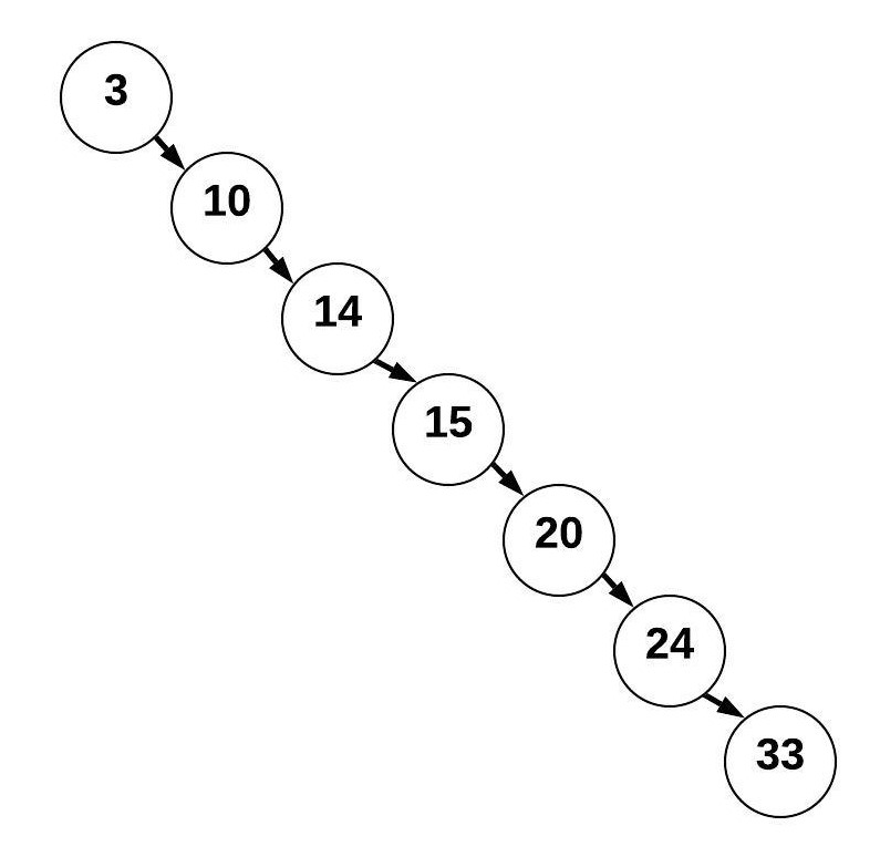
This tree is a BST but looks more like a linked list. This BST is unbalanced has a resulting performance for searching of O(n) instead of O(log n).
Balanced Binary Search Trees
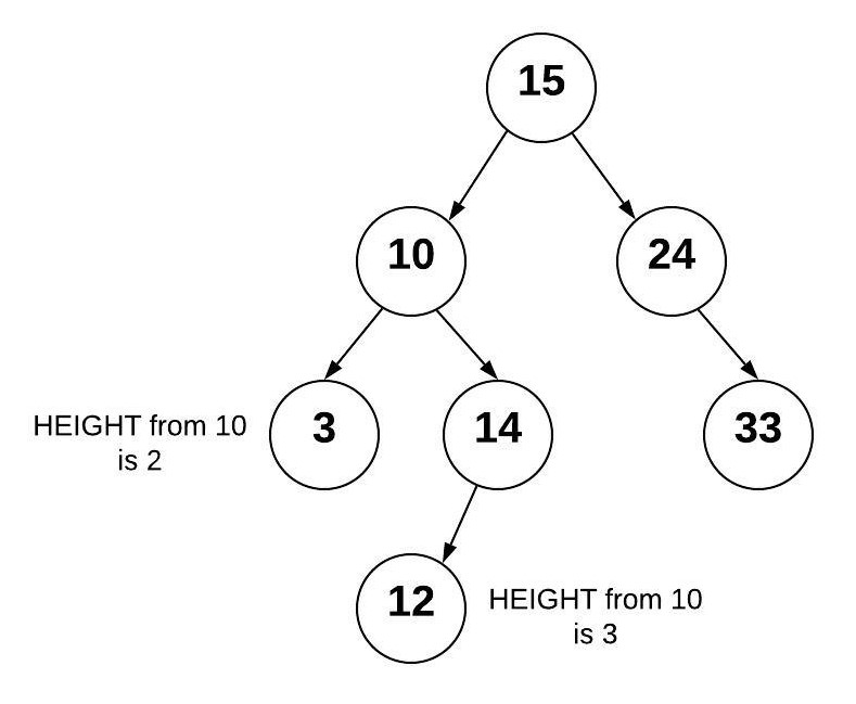
A balanced binary search tree (balanced BST) is a BST such that the difference of height between any two subtrees is not dramatically different. The height of a tree can be found by counting the maximum number of nodes between root and the leaves. Since it is not reasonable to expect that the order of data will result in a balanced BST, numerous algorithms have been written to detect if a tree is unbalanced and to correct the unbalance. Common algorithms include red black trees and AVL (Adelson-Velskii and Landis) trees. The example below shows an AVL tree which is balanced because the difference of height between subtrees is less than 2.
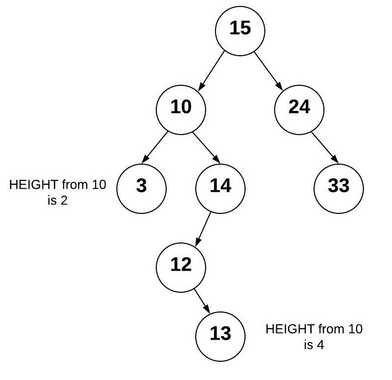
If we add 13 to the right of the 12, we end up with an unbalanced AVL tree because the height of the right subtree from 10 is now 2 more than the left subtree.
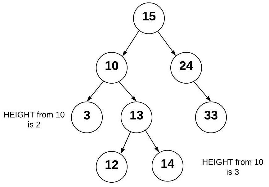
The AVL algorithm will detect that the tree has become unbalanced. To balance the tree, a node rotation will be performed. For our tree, we can rotate the node with 13 so that nodes 12 and 14 are children nodes of the 13. When this rotation is done, the tree returns to a balanced state. An AVL tree will always be a Balanced BST and therefore benefit from O(log n) performance.
BST Operations
BST operations can be very complicated (balanced BST's offering even more complication). We will look at two operations in our study of trees: inserting and traversing.
Inserting into a BST
Inserting into a BST is a recursive operations:
Smaller problem: Insert a value into either the left subtree or the right subtree based on the value.
Base case: If there is space to add the node (the subtree is empty), then the correct place has been found and the item can be inserted.
The code for inserting into a BST is shown below. Some things to note are as follows:
A node is defined as an object (in this example) of class
BST.Node. This is similar to what we saw with the linked list class. TheNodeclass is called an inner class because it's defined inside theBSTclass. The Node class contains three things:data(the value),left(pointer to the left node), andright(pointer to the right node).There are two functions. The
insertfunction is the one called by the user who wants to insert a value into the tree. This function is used to call the recursive function_insertstarting at the root node. As a special case, if the root node is empty (none), then we will put the new node in the root without using any recursion. We will follow this pattern for many of the recursive functions we write for the BST.In the
_insertfunction, we should identify the base case and the recursive calls to the correct subtrees.
def insert(self, data):
	"""
	Insert 'data' into the BST.  If the BST
	is empty, then set the root equal to the new
	node.  Otherwise, use _insert to recursively
	find the location to insert.
	"""
	if self.root is None:
		self.root = BST.Node(data)
	else:
		self._insert(data, self.root)  # Start at the root

def _insert(self, data, node):
	"""
	This function will look for a place to insert a node
	with 'data' inside of it.  The current subtree is
	represented by 'node'.  This function is intended to be
	called the first time by the insert function.
	"""
	if data < node.data:
		# The data belongs on the left side.
		if node.left is None:
			# We found an empty spot
			node.left = BST.Node(data)
		else:
			# Need to keep looking.  Call _insert
			# recursively on the left subtree.
			self._insert(data, node.left)
	elif data >= node.data:
		# The data belongs on the right side.
		if node.right is None:
			# We found an empty spot
			node.right = BST.Node(data)
		else:
			# Need to keep looking.  Call _insert
			# recursively on the right subtree.
			self._insert(data, node.right)
Traversing a BST
We traverse a BST when we want to display all the data in the tree. An in-order traversal will visit each node from smallest to largest. A similair process can be followed to visit each node from the largest to the smallest. This is also a recursive process:
Smaller problem: Traverse the left subtree of a node, use the current node, and then traverse the right subtree of the node.
Base case: If the subtree is empty, then don't recursively traverse or use anything.
The code for traversing a BST is shown below. In addition to the observations made to the insert code above, we should note the following additional things about this algorithm:
The starting function is called
__iter__. The use of double underscores in Python means that this function is part of the Python framework. When we write code likefor item in collection, the__iter__function is called on thecollectionto get the next item. In our case, the__iter__will provide the user the next value in the BST. We call this a generator function.The
yieldcommand is used to provide the next value to theforloop. Theyieldis like areturnstatement in a function. However, unlike areturn, theyieldwill allow the function to start back where it left off in the function when__iter__is called again. If we want delegate theyieldoperation to another function, the command is modified to beyield from. If a generator function (e.g.__iter__) needs to call another function which willyieldthe result, then we will need to use theyield fromkeywords.
def __iter__(self):
	"""
    Perform a forward traversal (in order traversal) starting from
    the root of the BST.  This is called a generator function.
    This function is called when a loop	is performed:

	for value in my_bst:
		print(value)

	"""
	yield from self._traverse_forward(self.root)  # Start at the root

def _traverse_forward(self, node):
	"""
	Does a forward traversal (in-order traversal) through the
	BST.  If the node that we are given (which is the current
	subtree) exists, then we will keep traversing on the left
	side (thus getting the smaller numbers first), then we will
	provide the data in the current node, and finally we will
	traverse on the right side (thus getting the larger numbers last).

	The use of the 'yield' will allow this function to support loops
	like:

	for value in my_bst:
		print(value)

    The keyword 'yield' will return the value for the 'for' loop to
    use.  When the 'for' loop wants to get the next value, the code in
    this function will start back up where the last 'yield' returned a
    value.  The keyword 'yield from' is used when our generator function
    needs to call another function for which a `yield` will be called.
    In other words, the `yield` is delegated by the generator function
    to another function.

	This function is intended to be called the first time by
	the __iter__ function.
	"""
	if node is not None:
		yield from self._traverse_forward(node.left)
		yield node.data
		yield from self._traverse_forward(node.right)
A reverse traversal is frequently associated with the __reversed__ function in Python.
BST in Python
In your assignment this week you will be writing your own BST class. Python does not have a built-in BST class. However, there are packages that can be installed from other developers such as bintrees that provides implementations of the BST.The table below shows the common functions in a BST.
| Common BST Operation | Description | Performance |
|---|---|---|
| insert(value) | Insert a value into the tree. | O(log n) - Recursively search the subtrees to find the next available spot |
| remove(value) | Remove a value from the tree. | O(log n) - Recursively search the subtrees to find the value and then remove it. This will require some cleanup of the adjacent nodes. |
| contains(value) | Determine if a value is in the tree. | O(log n) - Recursively search the subtrees to find the value. |
| traverse_forward | Visit all objects from smallest to largest. | O(n) - Recursively traverse the left subtree and then the right subtree. |
| traverse_reverse | Visit all objects from largest to smallest. | O(n) - Recursively traverse the right subtree and then the left subtree. |
| height(node) | Determine the height of a node. If the height of the tree is needed, the root node is provided. | O(n) - Recursively find the height of the left and right subtrees and then return the maximum height (plus one to account for the root). |
| size() | Return the size of the BST. | O(1) - The size is maintained within the BST class. |
| empty() | Returns true if the root node is empty. This can also be done by checking the size for 0. | O(1) - The comparison of the root node or the size. |
Key Terms
AVL Tree - Adelson-Velskii and Landis Tree. A balanced binary search tree that is checked unbalanced height after every modification to the tree. If the tree is unbalanced, then pre-determined algorithms are used to balance the tree.
balanced - A tree is balanced if the the height of the tree from the root to each leaf is consistent for all subtrees. The measure of consistentency will vary between algorithms but usually does not exceed a height difference of 1.
balanced binary search tree - A binary search tree which is balanced or restructured to be balanced. A balanced binary search tree has O(log n) performance when searching.
binary search tree - A binary tree that puts data less than the root to the left and greater than the root to the right. This type of a tree enables searching algorithms to be efficient.
binary tree - A tree that has up to two children for each node.
child - A child is a node connected from a parent node.
leaf - A leaf is a node that has no children.
node - An entry in a tree that contains both the value and pointers to any children nodes.
parent - A parent is a node that connects to children nodes.
root - The first parent in a tree.
subtree - Subset of a tree made by selecting a node to be the root and including all the children from that node.
traverse - The process of visiting all nodes (and subsequently their values) in a tree. Used frequently with a binary search tree using recursion to start at the leaf node that contains the smallest value and going to the leaf node that contains the largest value.
trees - A data structure that starts with a root node and is subsequently connected to multiple nodes according to a relationship between the nodes. The tree does not have any circular loops or unconnected nodes.